A brief history of vector symbolic architectures

So far, we’ve used the term Hyperdimensional Computing (HDC) to describe how high-dimensional distributed representations can encode, compose, and retrieve information. As you read more about the field, though, you’ll also see the name Vector Symbolic Architectures (VSA) ¹ . The names grew out of different research traditions, but today they refer to the same field.

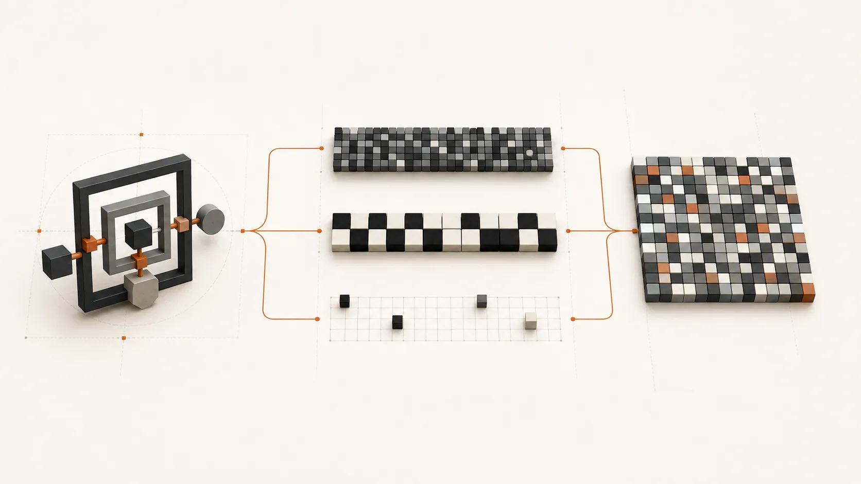
How can a wide, distributed representation preserve structure in the data? Across more than 30 years of work, HDC/VSA researchers have followed three broad routes to model data using the following types of hypervectors:

1. Dense, real-valued hypervectors: Models such as Holographic Reduced Representations (HRR), where every component can take a continuous value
2. Dense binary or bipolar hypervectors: Binary Spatter Codes (BSC) and Multiply-Add-Permute (MAP) models follow this approach, where every component takes one of two values (${0, 1}$ for binary, $\pm 1$ for bipolar)
3. Sparse hypervectors: Used by Sparse Binary Distributed Representations (SBDR) and sparse block codes, where only a small fraction of the components are non-zero

In this post, we’ll connect these historical arcs to the common HDC/VSA paradigms in use today, ending with MAP, the model we commonly use in our implementations, before showing how it can be implemented in just a few lines of PyTorch code.

The connectionist challenge: how to preserve structure?

In 1990, Geoffrey Hinton ² pointed to a hard problem for connectionist networks: a distributed pattern could represent an object, but how should it represent an object made of related parts?

A symbolic program handles this with nested records. A sentence can contain phrases, a plan can contain steps, and a visual scene can contain objects made of smaller objects. Fields and pointers keep each part attached to its role.

Connectionist networks don’t have those explicit fields or pointers. Their strength comes from spreading information across many units and reusing those units across representations. Hinton’s challenge was to keep that strength while meeting three requirements:

1. Represent the whole structure at once
2. Retain its parts and the roles they occupy
3. Reuse the same fixed network for structures of different shapes and sizes

Hinton and the wider connectionist field pursued these requirements through the neural-network architectures we’re no doubt very familiar with today. HDC/VSA researchers took a different route by designing the representations and algebra directly.

Does binding remain inside the original space?

Around the same time in 1990, Paul Smolensky ³ turned the connectionist network challenge into a binding problem. He introduced Tensor Product Representations (TPR), in which a role and value are each represented by a $D$-dimensional hypervector, and then combined with an outer product:

$$\mathbf{f}_{\text{name}} = \mathbf{r}_{\text{name}} \otimes \mathbf{v}_{\text{Maya}} = \mathbf{r}_{\text{name}}\mathbf{v}_{\text{Maya}}^{\mathsf{T}} \in \mathbb{R}^{D \times D}$$

A fact about Maya is represented by binding the role of “name” to the value “Maya”. This pairs every component of the role with every component of the value, allowing the role to be used later to retrieve its value.

The issue with this is that composing two hypervectors into a fact creates a $D \times D$ matrix. Binding preserves the role-value structure, but the resulting representation leaves the original hypervector space. Could we do better?

In 1995, Tony Plate provided a solution with Holographic Reduced Representations (HRR) ⁴ . Circular convolution sums the wrapped diagonals of the outer-product matrix, folding its $D^2$ structure into a single hypervector of $D$ components. The result can then participate in the same binding operation again. Recovery is approximate because several interactions are folded together, but the representation stays in $\mathbb{R}^{D}$.

This was a significant development in the field, allowing the same hypervector space to be used for both roles and values, and for both binding and unbinding.

$$\text{Smolensky: } \mathbb{R}^{D}\times\mathbb{R}^{D} \longrightarrow \mathbb{R}^{D\times D}$$ $$\text{Plate: } \mathbb{R}^{D}\times\mathbb{R}^{D} \longrightarrow \mathbb{R}^{D}$$

Multiplicative binding

Plate’s use of circular convolution established a pattern that would spread across the field in the 1990s: binding should retain the result in the same $D$-dimensional space, returning another hypervector of the same dimension as its inputs.

$$\operatorname{bind}: \mathcal{H}_{D}\times\mathcal{H}_{D} \longrightarrow \mathcal{H}_{D}$$

Researchers then changed what each component contained and found simpler operations that preserved the same pattern. The most direct route to the model we use today began with binary hypervectors.

Binary Spatter Codes (BSC)

Pentti Kanerva’s 1997 paper ⁵ applied the same binding-bundling ideas to hypervectors made of bits (every component is either $0$ or $1$). In Binary Spatter Codes (BSC), circular convolution is replaced by bitwise exclusive OR (XOR), and bundling uses a majority vote.

XOR produces another $D$-bit hypervector and is its own inverse. Applying the same role again retrieves the value:

$$(\mathbf{a}\mathbin{\operatorname{XOR}}\mathbf{b}) \mathbin{\operatorname{XOR}}\mathbf{a} = \mathbf{b}$$

The larger ideas were the same as Plate’s HRR. Only the representation had changed from real values to bits, and circular convolution had become XOR. The roles of the operations also stayed the same: binding formed an association, bundling collected several associations, and every result remained $D$-dimensional.

Reducing the tensor product to element-wise multiplication

Ross Gayler’s key insight in 1998 ⁶ was that element-wise multiplication could provide a particularly simple fixed-width reduction of Smolensky’s tensor product. Where the outer product retains all $D^2$ interactions between two hypervectors, element-wise multiplication ($\odot$) retains its $D$ diagonal terms:

$$\mathbf{a}\odot\mathbf{b} = \operatorname{diag} \left( \mathbf{a}\mathbf{b}^{\mathsf{T}} \right) \in\mathbb{R}^{D}$$

Each output component therefore depends only on the two input components in the same position:

$$(\mathbf{a}\odot\mathbf{b})_k=a_kb_k$$

The bound result remains $D$-dimensional, no $D\times D$ tensor is created, and no components have to be rearranged as they are in circular convolution.

Using bipolar values ($\pm 1$) doesn’t change the behavior: this operation is equivalent to Kanerva’s XOR binding under a simple change of representation:

$$0\leftrightarrow +1, \qquad 1\leftrightarrow -1$$

Just like in BSC, each bipolar component is its own multiplicative inverse because $a_k^2=1$, so the same operation can perform binding and unbinding:

$$\operatorname{bind}(\mathbf{a},\mathbf{b}) = \mathbf{a}\odot\mathbf{b}, \qquad (\mathbf{a}\odot\mathbf{b})\odot\mathbf{a} = \mathbf{b}$$

With element-wise multiplication for binding and element-wise addition for bundling, Gayler had a simple algebra that could be implemented with ordinary array arithmetic and used to build larger structures in the same $D$-dimensional space.

Multiply-Add-Permute (MAP)

Element-wise multiplication and addition are excellent at encoding which hypervectors belong together. What they cannot encode by themselves is how those hypervectors were arranged. Both operations are commutative, so swapping the inputs produces the same result:

$$\mathbf{a}\odot\mathbf{b}=\mathbf{b}\odot\mathbf{a}, \qquad \mathbf{a}+\mathbf{b}=\mathbf{b}+\mathbf{a}$$

That’s fine for an unordered collection, but not for an ordered pair, a sequence, or a nested structure. Once two hypervectors are bound or bundled together, their positional information is gone, so multiple different arrangements can produce the same hypervector.

Gayler used the term “permutation” for the operation that gives each structural position a distinguishable form before composition. A fixed permutation $\rho_p$ rearranges the components without changing the hypervector’s dimensionality. Two swapped inputs can now produce different results because each position applies a different transformation:

$$\rho_1(\mathbf{a})\odot\rho_2(\mathbf{b}) \neq \rho_1(\mathbf{b})\odot\rho_2(\mathbf{a})$$

By 2003, Gayler was presenting permutation alongside binding and bundling as the Multiply-Add-Permute (MAP) ⁷ model:

$$\begin{aligned} \operatorname{bind}(\mathbf{a},\mathbf{b}) &= \mathbf{a}\odot\mathbf{b} && \text{Multiply} \\ \operatorname{bundle}(\mathbf{a},\mathbf{b}) &= \mathbf{a}+\mathbf{b} && \text{Add} \\ \operatorname{permute}_{p}(\mathbf{a}) &= \rho_p(\mathbf{a}) && \text{Permute} \end{aligned}$$

Today, these are considered “the three operations” of HDC/VSA that preserve dimensionality. The benefit of MAP is that it provides a clean algebra for building larger structures using simple primitives like bipolar arrays.

The sparse hypervector route

The dense models above assume that most or all components are active. During the 1990s, a separate line of work by Nicolai Kussul and Dmitri Rachkovskij explored distributed representations in which almost every component remained zero:

$$\mathbf{h}\in\{0,1\}^{D}, \qquad \lVert\mathbf{h}\rVert_0=s, \qquad s\ll D$$

Here, $s$ is the number of active components. Their indices can be stored compactly, while the sparse hypervectors themselves work naturally with sparse associative memories.

Rachkovskij’s 2001 account of Sparse Binary Distributed Representations (SBDR) used Context-Dependent Thinning (CDT) for binding. ⁸ The operation constructs a combined pattern, then thins it back to the target sparsity. Unlike dense XOR or multiplicative binding, the result can retain some overlap with its inputs while still encoding their association.

This was not a sparse optimization of MAP. It was another answer to the same question: which representation and algebra can preserve structure without leaving the original $D$-dimensional space?

Later, Sparse Block Codes (SBC) imposed more structure by dividing the hypervector into blocks with one active component in each block. Binding could then use circular convolution within each block, combining fixed-width circular binding with sparse representations. ⁹

The HDC/VSA family of approaches

Over the years, HDC/VSA researchers followed many routes to solve the same problems. Each architecture chooses an algebra that fits its hypervector space:

Family	Hypervector space	Binding and recovery	Bundling	What the choice adds
Tensor Product Representations (TPR)	Dense real roles and values	Outer product; recover by contraction	Addition	Keeps role-value structure explicit, but the bound representation grows to $D\times D$
Holographic Reduced Representations (HRR)	Dense real	Circular convolution; approximate recovery by correlation	Addition	Compresses an outer-product-like interaction back to $D$ components
Binary Spatter Codes (BSC)	Dense binary	XOR for both binding and recovery	Majority vote	Makes the algebra bitwise and self-inverse
Multiply-Add-Permute (MAP)	Dense bipolar	Component-wise multiplication for both binding and recovery	Addition, optionally thresholded	Expresses the core operations with ordinary array arithmetic
Sparse Binary Distributed Representations (SBDR)	Sparse binary	Context-dependent thinning	Disjunction followed by thinning	Preserves sparsity and can retain overlap with the inputs
Sparse Block Codes (SBC)	One active component per block	Block-wise circular convolution	Addition	Combines structured sparsity with fixed-width binding

Towards Kanerva’s landmark 2009 synthesis

In 2008, Magnus Sahlgren, Anders Holst, and Pentti Kanerva gave permutation a particularly clear application: representing word order ¹⁰ . They applied a different power of the same permutation $\rho$ at each position, then bundled the results:

$$\mathbf{s} = \sum_{i=1}^{n}\rho^{i}(\mathbf{x}_i)$$

The word hypervectors remained in the same space, but the position of each word now changed how it contributed to the sequence. This was one of the first clear examples of how permutation could encode structure and order in a distributed representation.

By the time Kanerva’s landmark 2009 paper↗ was published, the fields of HDC and VSA had largely converged in both their terminology and their treatment of permutation as a general “positional transformation” alongside binding and bundling (associative composition). Modern surveys use the combined label HDC/VSA, preserving both historical names without treating either research lineage as the canonical one.

In the vocabulary used today, Kanerva’s synthesis leaves us with the three operators of HDC:

1. Binding associates two hypervectors
2. Bundling collects several hypervectors into one representation
3. Permutation marks structural position by rearranging components

From HDC theory to implementation

The mathematics behind these different approaches can look intimidating at first glance: tensor products, circular convolution, and hypervector arithmetic over thousands of dimensions. However, both software and hardware have improved tremendously since the field’s early days. Modern tensor frameworks can apply the same simple operation across every component in parallel on a wide range of processors and accelerators. This makes it possible to implement HDC/VSA operations in a few lines of code, even for hypervectors with thousands of components.

These days, it’s common to implement binding, bundling, and permutation using MAP in a framework such as PyTorch. The clearest example comes from TorchHD’s internal implementation of MAPTensor↗ , where each HDC operator delegates to a simple PyTorch operation.

Binding is multiplication

TorchHD binds two MAP hypervectors with torch.mul, which multiplies matching components:

def bind(self, other: "MAPTensor") -> "MAPTensor":
    return torch.mul(self, other)

This is the element-wise product introduced above. Two $D$-dimensional inputs produce another $D$-dimensional hypervector, and no outer-product matrix is constructed.

Bundling is addition

Bundling is just as direct. TorchHD adds the matching components with torch.add:

def bundle(self, other: "MAPTensor") -> "MAPTensor":
    return torch.add(self, other)

The sum retains information from both inputs. TorchHD deliberately leaves this result unnormalized; an encoder can normalize or threshold it later when the next operation requires bipolar values.

Permutation is a cyclic shift

For MAP permutation, TorchHD uses torch.roll to shift the components along the final dimension:

def permute(self, shifts: int = 1) -> "MAPTensor":
    return torch.roll(self, shifts=shifts, dims=-1)

The operation changes where each component appears without changing the hypervector’s contents or dimensionality. Applying the opposite shift reverses it.

Conclusions

This post covered the rather long but necessary history behind modern HDC/VSA. The field did not emerge linearly as one complete theory. Over 30+ years, it grew from several independent research arcs, each exploring how distributed representations could encode and manipulate structured information.

The early days of the field were largely about overcoming one important constraint: how to compose $D$-dimensional hypervectors so that the result is another hypervector in the same space, without blowing up the representation into a different space.

$$\mathcal{H}_{D}\times\mathcal{H}_{D} \longrightarrow \mathcal{H}_{D}$$

Once multiplicative binding satisfied this constraint, operations became truly composable. Larger, more complex structures could be built, allowing us to model data in almost any domain. HRR, BSC, MAP, and the sparse approaches each use a different algebra to achieve this.

Interestingly, many independent bodies of research found the same structural limit: binding encodes the fact that hypervectors are associated, but does not retain how those hypervectors were arranged (because binding is typically commutative). Permutation emerged as a positional transformation that could preserve this missing structure.

The permutation operator deserves a much deeper look: in the next post, we’ll explore why permutation is necessary, explain how it encodes position, and walk through realistic examples of when it’s useful. Stay tuned for more!

Footnotes

1. Denis Kleyko, Dmitri A. Rachkovskij, Evgeny Osipov, and Abbas Rahimi use HDC/VSA throughout their survey and define both names as referring to this same family of computational models. See “A Survey on Hyperdimensional Computing aka Vector Symbolic Architectures, Part I: Models and Data Transformations”↗ . ↩

2. Geoffrey Hinton, “Mapping Part-Whole Hierarchies into Connectionist Networks”↗ (1990). Hinton’s paper considers how hierarchical structures found in sentences, plans, and visual scenes can be mapped onto the fixed hardware of a connectionist network. ↩

3. Paul Smolensky, “Tensor Product Variable Binding and the Representation of Symbolic Structures in Connectionist Systems”↗ (1990). Smolensky defines tensor products as a distributed representation of role-value bindings that can be recursively composed into larger symbolic structures. ↩

4. Tony Plate, “Holographic Reduced Representations”↗ (1995). Plate uses circular convolution to keep binding within one hypervector space and circular correlation for approximate recovery. ↩

5. Pentti Kanerva, “The Spatter Code: Holographic Reduced Representation in the Binary Domain”↗ (1997). Kanerva uses dense binary hypervectors, XOR for binding and probing, and majority rule for bundling. ↩

6. Ross Gayler, “Multiplicative Binding, Representation Operators & Analogy”↗ (1998). Gayler relates component-wise multiplicative binding to both Kanerva’s XOR binding and Plate’s compressed tensor-product construction. ↩

7. Ross Gayler, “Vector Symbolic Architectures Answer Jackendoff’s Challenges for Cognitive Neuroscience”↗ (2003). Gayler describes VSA models through multiplication-like, addition-like, and permutation-like operations, using MAP as a concrete example. ↩

8. Dmitri A. Rachkovskij, “Representation and Processing of Structures with Binary Sparse Distributed Codes”↗ (2001). Rachkovskij describes fixed-dimensional sparse binary representations, context-dependent thinning, and shift permutations for structured data. ↩

9. E. Paxon Frady, Denis Kleyko, and Friedrich T. Sommer, “Variable Binding for Sparse Distributed Representations: Theory and Applications”↗ (published online in 2021; journal issue in 2023). The authors study block-local circular convolution for sparse block codes. ↩

10. Magnus Sahlgren, Anders Holst, and Pentti Kanerva, “Permutations as a Means to Encode Order in Word Space”↗ (2008). The paper encodes sequence information in fixed-width hypervectors by applying coordinate permutations according to word position. ↩